From raw linelist data to Re estimates
linelist_workflow_example.RmdIn this vignette, we demonstrate a workflow for estimating Re from a linelist.
library(estimateR)

# Data handling packages
library(dplyr)
#>
#> Attaching package: 'dplyr'
#> The following objects are masked from 'package:stats':
#>
#>     filter, lag
#> The following objects are masked from 'package:base':
#>
#>     intersect, setdiff, setequal, union
library(tidyr)

# Package for plotting
library(ggplot2)
The example data is a synthetic version of a linelist of COVID-19 cases. The aggregated incidence of this linelist corresponds to or closely matches the incidence of Swiss cases as reported by the Federal Office of Public Health. To keep the data handling fast and easy, we restricted the simulated data from February to June 2020. The data is stored in the CH_simulated_linelist variable.
# Simulated Swiss linelist
head(CH_simulated_linelist, n = 10)
#> # A tibble: 10 × 2
#>    confirmation_date symptom_onset_date
#>    <date>            <date>
#>  1 2020-02-24        NA
#>  2 2020-02-25        NA
#>  3 2020-02-26        NA
#>  4 2020-02-26        2020-02-17
#>  5 2020-02-26        NA
#>  6 2020-02-26        NA
#>  7 2020-02-26        NA
#>  8 2020-02-26        NA
#>  9 2020-02-26        NA
#> 10 2020-02-26        NA
Data preparation
Aggregated incidence
We start by transforming the linelist into a dataframe that contains the daily incidence for case confirmations. When doing so, we make sure to extract as much information as possible from the linelist in order to better inform the Re estimation. For some cases recorded in the linelist, the date of onset of symptom is known. For these cases, inferring the date of infection is easier than cases for which this information was not recorded. -We assume that all recorded cases are symptomatic, and that tests are always performed after the onset of symptoms- The delayed observation of the infection event is less delayed when it is the onset of symptoms rather than the case confirmation. Therefore, we will separate cases in two incidences: 1.cases for which the date of symptom onset is known. In that case, the incidence vector represents these onset events. 1.cases with no known date of symptom onset. In that case, the incidence vector represents case confirmation events.
First, we construct the incidence of events of onset of symptoms for cases for which it is known.
onset_incidence <- CH_simulated_linelist %>%
  transmute(date = symptom_onset_date) %>%
  filter(!is.na(date)) %>%
  group_by(date) %>%
  tally(name = "onset_incidence")

head(onset_incidence)
#> # A tibble: 6 × 2
#>   date       onset_incidence
#>   <date>               <int>
#> 1 2020-02-17               2
#> 2 2020-02-18               1
#> 3 2020-02-19               1
#> 4 2020-02-20               3
#> 5 2020-02-21               4
#> 6 2020-02-22               2
Then, we construct the incidence of events of case confirmation with no known symptom onset date.
confirmation_incidence <- CH_simulated_linelist %>%
  # only keep report_date when we do not have the onset_date
  mutate(confirmation_date = if_else(is.na(symptom_onset_date), confirmation_date, as.Date(NA))) %>%
  transmute(date = confirmation_date) %>%
  filter(!is.na(date)) %>%
  group_by(date) %>%
  tally(name = "confirmation_incidence")

head(confirmation_incidence)
#> # A tibble: 6 × 2
#>   date       confirmation_incidence
#>   <date>                      <int>
#> 1 2020-02-24                      1
#> 2 2020-02-25                      1
#> 3 2020-02-26                      9
#> 4 2020-02-27                      8
#> 5 2020-02-28                      6
#> 6 2020-02-29                      8
Now let us merge the two into a single dataframe. We need to make sure we align the two incidence vectors, and fill the missing dates with zero values.
CH_incidence_data <- full_join(onset_incidence, confirmation_incidence, by = 'date') %>%
  replace_na(list(onset_incidence = 0, confirmation_incidence = 0)) %>%
  complete(date = seq.Date(min(date), # add zeroes for dates with no reported case
                  max(date),
                  by = "days"),
                  fill = list(onset_incidence = 0,
                              confirmation_incidence = 0)) %>%
  select(date, onset_incidence, confirmation_incidence) %>%
  arrange(date)

head(CH_incidence_data)
#> # A tibble: 6 × 3
#>   date       onset_incidence confirmation_incidence
#>   <date>               <dbl>                  <dbl>
#> 1 2020-02-17               2                      0
#> 2 2020-02-18               1                      0
#> 3 2020-02-19               1                      0
#> 4 2020-02-20               3                      0
#> 5 2020-02-21               4                      0
#> 6 2020-02-22               2                      0
Delay data
As a second step, we make use of the linelist to inform the analysis on the distribution of the delay between onset of symptom and case confirmation. This lets us use empirical distribution for delays instead of estimates of delays from the literature, which may not be as relevant to the particular data of interest. Moreover, providing this data allows estimateR to let the empirical delay distributions vary through time, instead of relying on a single average estimate for the entire time window.
CH_delay_data <- CH_simulated_linelist %>%
  filter(!is.na(symptom_onset_date), !is.na(confirmation_date)) %>%
  transmute(event_date = symptom_onset_date,
            report_date = confirmation_date) %>%
  mutate(report_delay = as.integer(report_date - event_date)) %>%
  mutate(report_delay = if_else(report_delay < 0, as.integer(NA), report_delay)) %>%  # curate negative delays
  filter(!is.na(report_delay)) %>% # remove NA values
  select(-report_date) %>% # rearrange dataset
  arrange(event_date)

head(CH_delay_data)
#> # A tibble: 6 × 2
#>   event_date report_delay
#>   <date>            <int>
#> 1 2020-02-17            9
#> 2 2020-02-17           14
#> 3 2020-02-18           17
#> 4 2020-02-19           21
#> 5 2020-02-20            8
#> 6 2020-02-20            9
Analysis
Additional user input
Additionally to the incidence and delay data prepared in the section above, we need to specify the incubation period for COVID-19 and the serial interval.
# Delay between infection and onset of symptoms (incubation period) in days
# Ref: Linton et al., Journal of Clinical Medicine, 2020
# Gamma distribution parameter
shape_incubation <- 3.2
scale_incubation <- 1.3

# Incubation period delay distribution
distribution_incubation <- list(name = "gamma",
                                shape = shape_incubation,
                                scale = scale_incubation)

# Serial interval (for Re estimation) in days
# Ref: Nishiura et al.,International Journal of Infectious Diseases, 2020
mean_serial_interval <- 4.8
std_serial_interval <- 2.3
Now, we set some parameter of the analysis:
estimation_window = 3 # 3-day sliding window for the Re estimation
minimum_cumul_incidence = 100 # we start estimating Re after at least 100 cases have been recorded
N_bootstrap_replicates = 100 # we take 100 replicates in the bootstrapping procedure

# We specifiy the reference date (first date of data) and the time step of data.
ref_date = min(CH_incidence_data$date)
time_step = "day"
Computation
We can then perform the Re estimation. The computation should take a few seconds to complete.
CH_estimates <- get_bootstrapped_estimates_from_combined_observations(
partially_delayed_incidence = CH_incidence_data$onset_incidence,
fully_delayed_incidence = CH_incidence_data$confirmation_incidence,
N_bootstrap_replicates = N_bootstrap_replicates,
delay_until_partial = distribution_incubation,
delay_until_final_report = CH_delay_data,
partial_observation_requires_full_observation = TRUE,
combine_bootstrap_and_estimation_uncertainties = TRUE,
estimation_window = estimation_window,
minimum_cumul_incidence = minimum_cumul_incidence,
mean_serial_interval = mean_serial_interval,
std_serial_interval = std_serial_interval,
ref_date = ref_date,
time_step = time_step
)
head(CH_estimates)
#> # A tibble: 6 × 4
#> date Re_estimate CI_down_Re_estimate CI_up_Re_estimate
#> <date> <dbl> <dbl> <dbl>
#> 1 2020-02-23 3.16 2.66 3.71
#> 2 2020-02-24 3.16 2.36 3.95
#> 3 2020-02-25 3.13 0.801 5.46
#> 4 2020-02-26 3.09 1.70 4.48
#> 5 2020-02-27 3.04 2.53 3.55
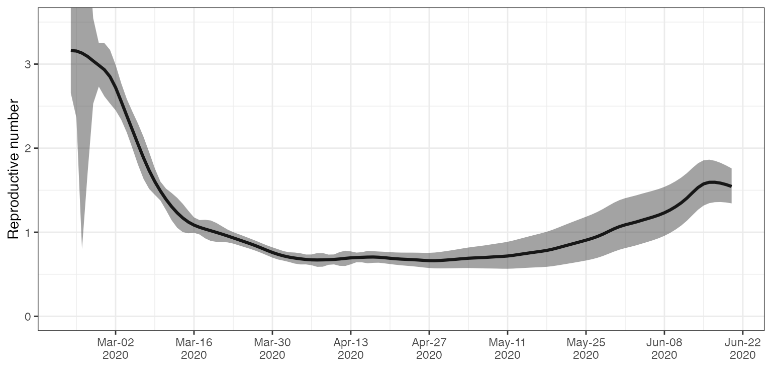
#> 6 2020-02-28 2.99 2.73 3.25Plot
ggplot(CH_estimates, aes(x = date, y = Re_estimate)) +
  geom_line(lwd=  1.1) +
  geom_ribbon(aes(x = date, ymax = CI_up_Re_estimate, ymin = CI_down_Re_estimate), alpha = 0.45, colour = NA) +
  scale_x_date(date_breaks = "2 weeks",
               date_labels = '%b-%d\n%Y') +
  ylab("Reproductive number") +
  coord_cartesian(ylim = c(0, 3.5)) +
  xlab("") +
  theme_bw()