estimateR
estimateR.RmdThis vignette’s purpose is to demonstrate how to use the estimateR package in a simple use case. The estimateR package provides tools to estimate the effective reproductive number through time from delayed and indirect observations of infection events.
Let us start with a toy dataset. We will assume in this example that the incidence data represents daily counts of case confirmations. This incidence data counts the number of people getting tested positive for a particular infectious disease X on day T.
library(estimateR)

toy_incidence_data <- c(
  4, 9, 19, 14, 36, 16, 39, 27, 46,
  77, 78, 113, 102, 134, 165, 183,
  219, 247, 266, 308, 304, 324, 346,
  348, 331, 311, 267, 288, 254, 239
)
Here, we represent the incidence data in its simplest form: a numeric vector. Let us assume reporting started on Feb 24th 2021. There are 30 entries in our toy_incidence_data vector, each representing data for a single day in succession. Thus, there were 4 reported cases on Feb 24th and 239 on March 25th, the last reporting date.
Smoothing
The toy incidence data we generated above is noisy, as real incidence data could be. Therefore, we start by smoothing the toy data, using the LOESS smoothing method.
smoothed_toy_incidence <- smooth_incidence(
  incidence_data = toy_incidence_data,
  smoothing_method = "LOESS"
)
To estimate the effective reproductive number through time Re, we need the time series (in the conceptual sense, not the data type sense) of infection events over the period of interest. But all we have at the moment is a smoothed version of the time series of confirmed case reports. There are two major differences between this time series and the time series of infection events. First, in almost all real-life cases, only a fraction of infected individuals will get tested, and even among individuals tested some false-negative results will arise. For simplicity, we ignore false-positive numbers here. This difference does not cause direct issues for estimating Re. Indeed, as long as the fraction of tested individuals among the pool of newly-infected individuals remains constant then Re estimates are not biased.
Second, a case-confirmation report is not a direct observation of an infection event. This report comes with a delay. For simplicity, we assume here that individuals are only tested after they start showing symptoms for the pathogen of interest. The delay between infection and observation can thus be divided into two distinct time periods: the incubation period and the delay from symptom onset to case confirmation. The exact number of days this delay represents will vary from individual to individual, we capture this variability by assuming the delay observed in any particular individual is the result of a random draw from a probability distribution representing the population variability in the reporting delays.
In mathematical terms, the observed time series is the result of the convolution of the time series of infections and the distribution of delays. To infer the time series of infection events, we perform the inverse transformation: we deconvolve the delay distribution from the time series of observations. We use the Richardson-Lucy algorithm to perform this deconvolution step.
In estimateR, we approximate both delay distributions -incubation period and delay from onset of symptoms to case observation- by gamma distributions.
Inference of infection events
# These numbers are part of the user input, they need to be adapted to the particular disease studied.
# The values chosen below are arbitrary.

# Incubation period - gamma distribution parameters
shape_incubation <- 3.2
scale_incubation <- 1.3
incubation <- list(name="gamma", shape = shape_incubation, scale = scale_incubation)

# Delay from onset of symptoms to case observation - gamma distribution parameters
shape_onset_to_report <- 2.7
scale_onset_to_report <- 1.6
onset_to_report <- list(name="gamma", shape = shape_onset_to_report, scale = scale_onset_to_report)

# Infer the original infection events by deconvolving the delays from the smoothed observations.
toy_infection_events <- deconvolve_incidence(
  incidence_data = smoothed_toy_incidence,
  deconvolution_method = "Richardson-Lucy delay distribution",
  delay = list(incubation, onset_to_report)
)
Reproductive number estimation
Now, we can estimate the effective reproductive number. We do so using a wrapper around the EpiEstim package. As additional input, we need the mean and standard deviation of the serial interval of the disease of interest.
# We specify these parameters in the same unit as the time steps in the original observation data.
# For instance, if the original data represents daily reports, the parameters below must be specified in days
# (this is the case in this toy example).
mean_serial_interval <- 4.8
std_serial_interval <- 2.3

estimation_window <- 3
# The estimation window corresponds to the size of the sliding window used in EpiEstim.
# See help(estimate_Re) for additional details.
# Here, it is set to three days.

toy_Re_estimates <- estimate_Re(
  incidence_data = toy_infection_events,
  estimation_method = "EpiEstim sliding window",
  estimation_window = estimation_window,
  mean_serial_interval = mean_serial_interval,
  std_serial_interval = std_serial_interval
)
Final result
Finally, we merge the outputs of the different steps into a dataframe, along with a column for dates.
toy_results <- merge_outputs(
  list(
    "observed_incidence" = toy_incidence_data, # The LHS terms are arbitrary names for the output of each step.
    "smoothed_incidence" = smoothed_toy_incidence,
    "deconvolved_incidence" = toy_infection_events,
    "Re_estimate" = toy_Re_estimates
  ),
  ref_date = as.Date("2020-02-24"), # The observation data starts on Feb 24th 2021.
  time_step = "day"
)

head(toy_results)
#>         date observed_incidence smoothed_incidence deconvolved_incidence
#> 1 2020-02-16                 NA                 NA              15.64136
#> 2 2020-02-17                 NA                 NA              18.89345
#> 3 2020-02-18                 NA                 NA              22.53378
#> 4 2020-02-19                 NA                 NA              27.04901
#> 5 2020-02-20                 NA                 NA              32.96153
#> 6 2020-02-21                 NA                 NA              40.69800
#>   Re_estimate
#> 1          NA
#> 2          NA
#> 3          NA
#> 4          NA
#> 5          NA
#> 6          NA
Simplification using a wrapper function
The process presented above can be performed in a single function estimate_Re_from_noisy_delayed_incidence. We rewrite all the code blocks above using estimate_Re_from_noisy_delayed_incidence this time.
date_first_data_point <- as.Date("2020-02-24")
toy_incidence_data <- c(
  4, 9, 19, 14, 36, 16, 39, 27, 46,
  77, 78, 113, 102, 134, 165, 183,
  219, 247, 266, 308, 304, 324, 346,
  348, 331, 311, 267, 288, 254, 239
)

# Incubation period - gamma distribution parameters
shape_incubation <- 3.2
scale_incubation <- 1.3
incubation <- list(name="gamma", shape = shape_incubation, scale = scale_incubation)

# Delay from onset of symptoms to case observation - gamma distribution parameters
shape_onset_to_report <- 2.7
scale_onset_to_report <- 1.6
onset_to_report <- list(name="gamma", shape = shape_onset_to_report, scale = scale_onset_to_report)

mean_serial_interval <- 4.8
std_serial_interval <- 2.3

estimation_window <- 3

toy_estimates <- estimate_Re_from_noisy_delayed_incidence(
  toy_incidence_data,
  smoothing_method = "LOESS",
  deconvolution_method = "Richardson-Lucy delay distribution",
  estimation_method = "EpiEstim sliding window",
  delay = list(incubation, onset_to_report),
  estimation_window = estimation_window,
  mean_serial_interval = mean_serial_interval,
  std_serial_interval  = std_serial_interval,
  output_Re_only = FALSE,
  ref_date = date_first_data_point,
  time_step = "day"
)

head(toy_estimates)
#>         date observed_incidence smoothed_incidence deconvolved_incidence
#> 1 2020-02-16                 NA                 NA              15.64136
#> 2 2020-02-17                 NA                 NA              18.89345
#> 3 2020-02-18                 NA                 NA              22.53378
#> 4 2020-02-19                 NA                 NA              27.04901
#> 5 2020-02-20                 NA                 NA              32.96153
#> 6 2020-02-21                 NA                 NA              40.69800
#>   Re_estimate
#> 1          NA
#> 2          NA
#> 3          NA
#> 4          NA
#> 5          NA
#> 6          NA
Uncertainty estimation
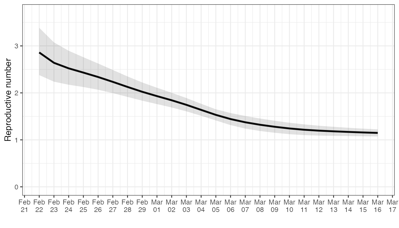
In order to estimate the uncertainty around the Re estimation made above, we apply a bootstrapping procedure to the toy observation data. This procedure produces a number of so-called bootstrap samples from the original observations. By re-estimating Re with each of these artificial time series, we can approximate the uncertainty in Re estimates that derives from the noise in the original data.
N_bootstrap_replicates <- 100

estimates <- get_block_bootstrapped_estimate(toy_incidence_data,
  N_bootstrap_replicates = N_bootstrap_replicates,
  smoothing_method = "LOESS",
  deconvolution_method = "Richardson-Lucy delay distribution",
  estimation_method = "EpiEstim sliding window",
  uncertainty_summary_method = "original estimate - CI from bootstrap estimates",
  combine_bootstrap_and_estimation_uncertainties = TRUE,
  delay = list(incubation, onset_to_report),
  estimation_window = estimation_window,
  mean_serial_interval = mean_serial_interval,
  std_serial_interval = std_serial_interval,
  ref_date = as.Date("2020-02-24"),
  time_step = "day"
)

head(estimates)
#> # A tibble: 6 × 4
#>   date       Re_estimate CI_down_Re_estimate CI_up_Re_estimate
#>   <date>           <dbl>               <dbl>             <dbl>
#> 1 2020-02-22        2.86                2.38              3.39
#> 2 2020-02-23        2.64                2.24              3.08
#> 3 2020-02-24        2.52                2.17              2.90
#> 4 2020-02-25        2.43                2.12              2.76
#> 5 2020-02-26        2.34                2.07              2.63
#> 6 2020-02-27        2.23                1.99              2.49
library(ggplot2)
ggplot(estimates, aes(x = date, y = Re_estimate)) +
  geom_line(lwd=  1.1) +
  geom_ribbon(aes(x = date, ymax = CI_up_Re_estimate, ymin = CI_down_Re_estimate), alpha = 0.15, colour = NA) +
  scale_x_date(date_breaks = "1 day",
               date_labels = '%b\n%d') +
  ylab("Reproductive number") +
  coord_cartesian(ylim = c(0, 3.7)) +
  xlab("") +
  theme_bw()